MAMU comes with the radar_cone function, originally
designed to interpolate data points around radar stations where birds
may be flying. For a given (x,y) spatial point, heading, and radius,
radar_cone produces a conical gradient raster.
library(MAMU)

# Generate a dummy point of data somewhere in British Columbia
pt <- sf::st_point(c(-126, 53)) %>%
  sf::st_sfc(crs = 4326) %>%
  sf::st_transform(crs = 3005)

# Set our radius, flight heading, and raster resolution parameters
radius <- 30000
heading <- 45
res <- 500

# Create a set of maximum raster values
max_values <- c(1, 5, 10)

# Create a set of pie chunks to interpolate around
# to demonstrate what the 'theta' parameter does in the function
thetas <- c(0, 30, 90, 120)

# Now create a few sets of interpolated cones!
# For each value of theta, run the radar_cone function
# with our above parameters.
cones_max1 <- mapply(radar_cone,
       theta = thetas,
       MoreArgs = list(pt = pt,
                       radius = radius,
                       res = res,
                       heading = heading,
                       invert = TRUE,
                       maxvalue = max_values[[1]]))

cones_max5 <- mapply(radar_cone,
       theta = thetas,
       MoreArgs = list(pt = pt,
                       radius = radius,
                       res = res,
                       heading = heading,
                       invert = TRUE,
                       maxvalue = max_values[[2]]))

cones_max10 <- mapply(radar_cone,
       theta = thetas,
       MoreArgs = list(pt = pt,
                       radius = radius,
                       res = res,
                       heading = heading,
                       invert = TRUE,
                       maxvalue = max_values[[3]]))
par(mfrow = c(3, 4), oma=c(2,2,0,0))

{
terra::plot(cones_max1[[1]], range = c(0,rev(max_values)[1])) # max value 1; theta = 0
terra::plot(cones_max1[[2]], range = c(0,rev(max_values)[1])) # max value 1; theta = 30°
terra::plot(cones_max1[[3]], range = c(0,rev(max_values)[1])) # max value 1; theta = 90°
terra::plot(cones_max1[[4]], range = c(0,rev(max_values)[1])) # max value 1; theta = 120°

terra::plot(cones_max5[[1]], range = c(0,rev(max_values)[1])) # max value 5; theta = 0
terra::plot(cones_max5[[2]], range = c(0,rev(max_values)[1])) # max value 5; theta = 30°
terra::plot(cones_max5[[3]], range = c(0,rev(max_values)[1])) # max value 5; theta = 90°
terra::plot(cones_max5[[4]], range = c(0,rev(max_values)[1])) # max value 5; theta = 120°

terra::plot(cones_max10[[1]], range = c(0,rev(max_values)[1])) # max value 10; theta = 0
terra::plot(cones_max10[[2]], range = c(0,rev(max_values)[1])) # max value 10; theta = 30°
terra::plot(cones_max10[[3]], range = c(0,rev(max_values)[1])) # max value 10; theta = 90°
terra::plot(cones_max10[[4]], range = c(0,rev(max_values)[1])) # max value 10; theta = 120°
}

mtext("Maximum value (1, 5, 10)",side=2,line=0,outer=TRUE,cex=1.3)
mtext("Wedge size (NA, 1/12, 1/4, 1/3)",side=1,line=0,outer=TRUE,cex=1.3,las=0)
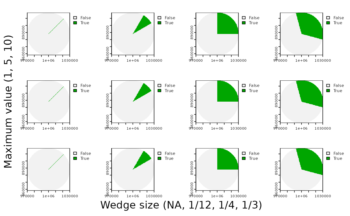
par(mfrow = c(3, 4), oma=c(2,2,0,0))

terra::plot(cones_max1[[1]] == 0) # max value 1; theta = 0
terra::plot(cones_max1[[2]] == 0) # max value 1; theta = 30°
terra::plot(cones_max1[[3]] == 0) # max value 1; theta = 90°
terra::plot(cones_max1[[4]] == 0) # max value 1; theta = 120°

terra::plot(cones_max5[[1]] == 0) # max value 5; theta = 0
terra::plot(cones_max5[[2]] == 0) # max value 5; theta = 30°
terra::plot(cones_max5[[3]] == 0) # max value 5; theta = 90°
terra::plot(cones_max5[[4]] == 0) # max value 5; theta = 120°

terra::plot(cones_max10[[1]] == 0) # max value 10; theta = 0
terra::plot(cones_max10[[2]] == 0) # max value 10; theta = 30°
terra::plot(cones_max10[[3]] == 0) # max value 10; theta = 90°
terra::plot(cones_max10[[4]] == 0) # max value 10; theta = 120°

mtext("Maximum value (1, 5, 10)",side=2,line=0,outer=TRUE,cex=1.3)
mtext("Wedge size (NA, 1/12, 1/4, 1/3)",side=1,line=0,outer=TRUE,cex=1.3,las=0)